The integrated rate law of a chemical reaction shows how the concentrations of reactants change with time. For example, you are running a reaction and want to what the concentration of reactant A will be in 1 hour, how long it will take to produce 2 moles of a product and etc.
The integrated rate law depends on the reaction order and is derived by taking the integral of the corresponding differential rate law.
We will cover this conversion in a short separate article, however, since you are most likely not going to need it, today’s focus will be on the integrated rate laws and their applications.
The Integrated Rate Law of a Zero-Order Reaction
Remember, for a simple hypothetical reaction where molecule A transforms into products, the (differential) rate law for a zero-order reaction can be written as:
A → Products
Rate = k[A]0 = k
Integrating the differential rate law, we obtain the integrated rate law for the zero-order reactions:
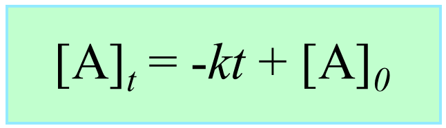
Note that the zero-order integrated rate law is also in the form of an equation for a straight line:
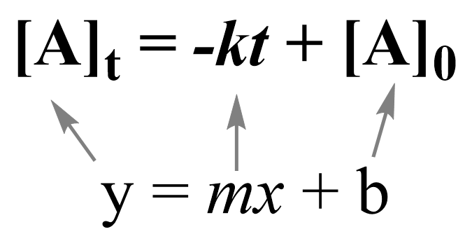
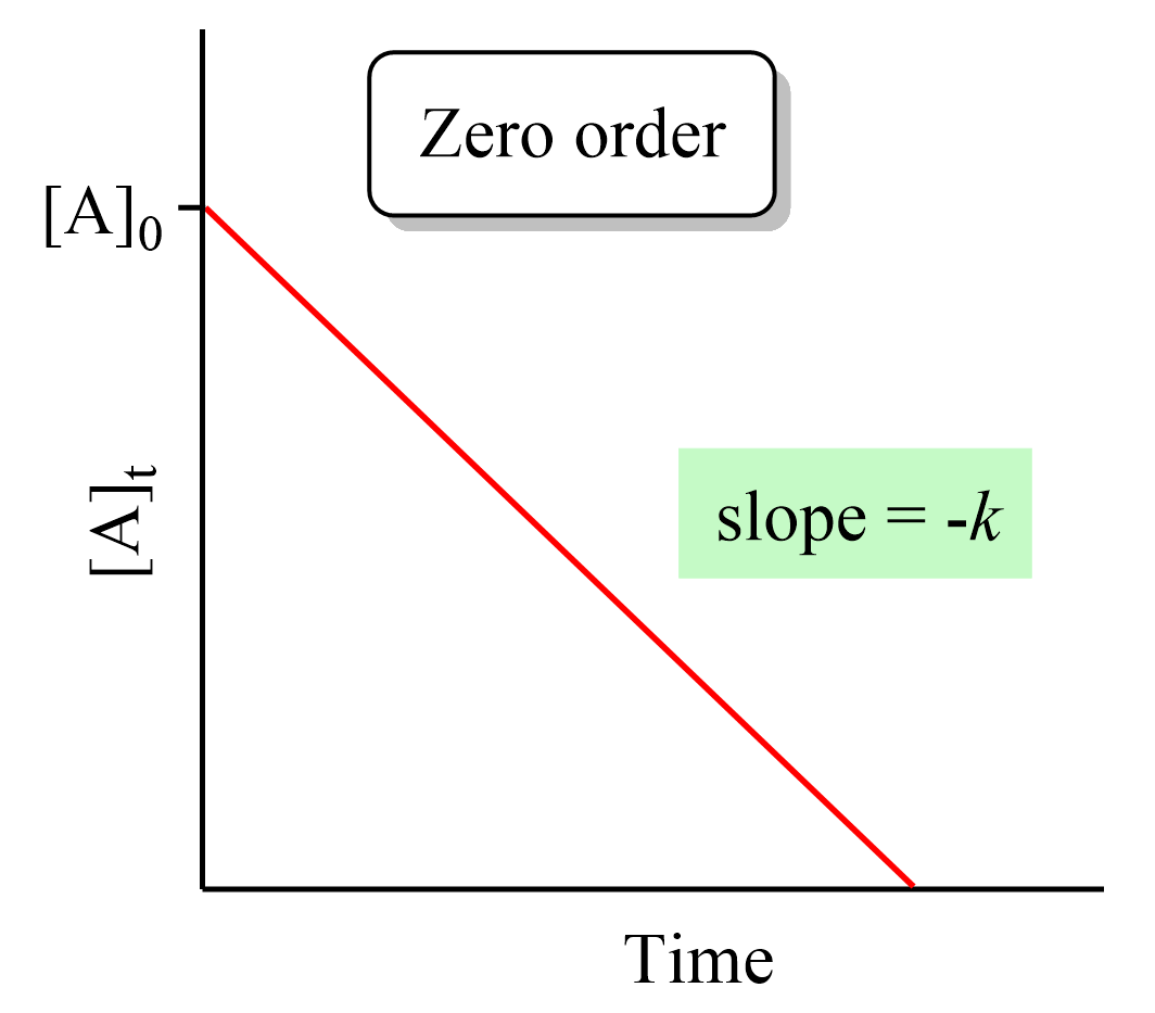
Therefore, a straight line with a slope of –k and an intercept of [A]0 is obtained in a graph of [A] versus time:
The Integrated Rate Law of a First-Order Reaction
The rate law for a simple first-order reaction can be written as:
A → Products
Rate = k[A]1
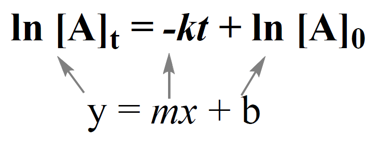
Integrating the differential rate law, we obtain the integrated rate law for the first-order reactions:
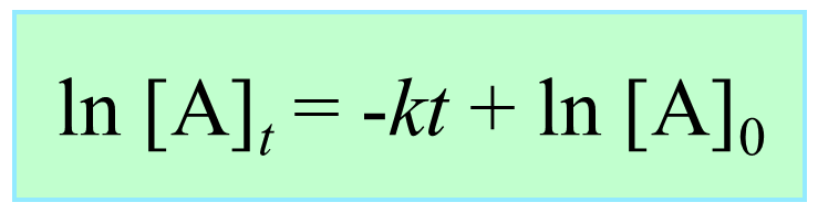
The integrated rate law for first-order reactions also has the form of an equation for a straight line. However, unlike the zero-order reaction, a graph of ln[A]t versus time yields a straight line with a slope of –k and a y-intercept of ln [A]0.
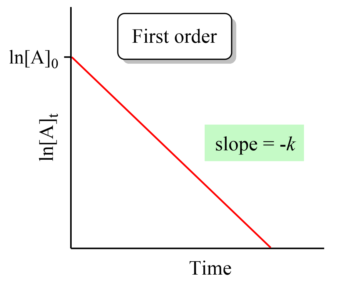
Notice that if we plot the concentration instead of its logarithm, an exponential decrease will be obtained. This is the strategy for determining the reaction order and thus the integrated rate low, which will cover in the next article.
The Integrated Rate Law of a Second-Order Reaction
A second-order reaction with one reactant appearing in the rate law can be represented as:
A → Products
Rate = k[A]2
Integrating the differential rate law, we obtain the integrated rate law for the first-order reactions:
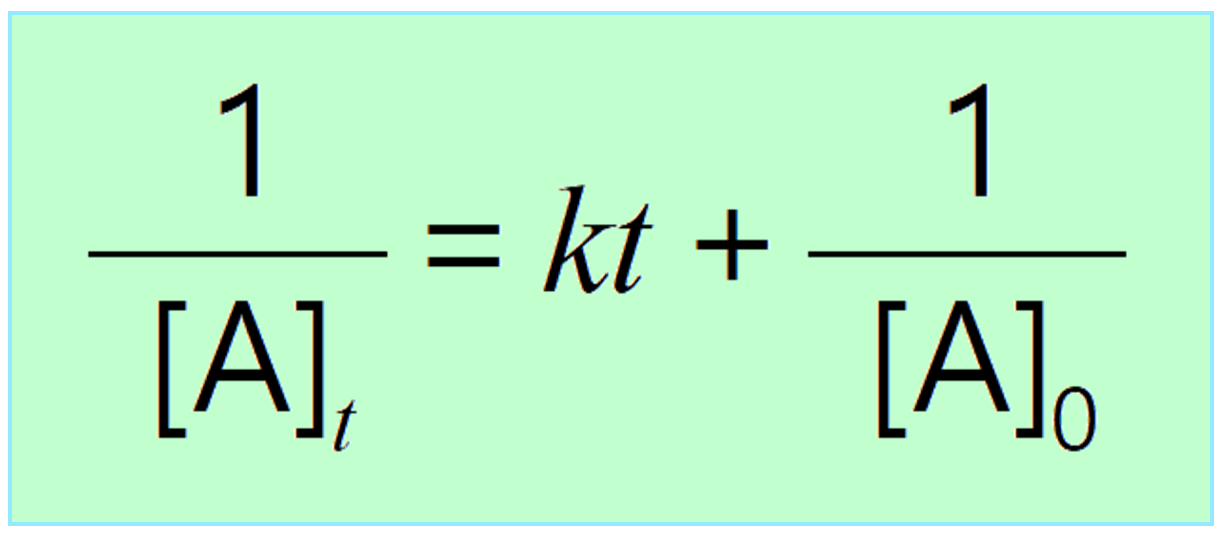
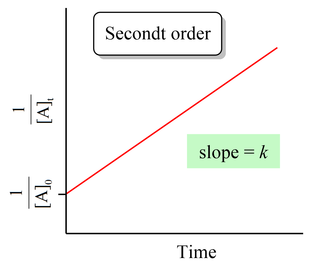
Just like the zero- and first-order reactions, the integrated rate law of second-order reaction is also in the form of a straight line where the 1/[A]t versus time yields a straight line with a slope of k and a y-intercept of 1/[A]0.
How do we use the integrated rate laws?
So, we have obtained the equation and the graph for the integrated rate laws, and the question is what do we use them for?
There are two main applications, at least two main types of problems, you will be given in your class based on the integrated rate laws:
- One is determining the concentration of a reactant or product at a certain point of the reaction when the reaction order is provided.
- The second is actually determining the rate law based on the data on how the concentration changes with time.
Let’s do an example of determining the concertation of a reactant when the reaction order is given.
Example:
Dinitrogen pentoxide, N2O5, decomposes by a first-order reaction according to the following equation:
2N2O5(g) → 2N2O4(g) + O2(g) k = 3.4 x 10⁻⁶/s
What would be the concentration of N2O5 after running the reaction for 3.00 hr if the initial concentration of N2O5 was 0.0465 mol/L?
Solution:
The integrated rate law for first-order reactions can be written as:
ln [A]t = –kt + ln [A]0
Let [N2O5]0 be 0.0465 M, and [N2O5]t be the concentration after 3.00 hr. Because the rate constant is expressed using seconds, 3.00 hr must be converted to seconds, which is 3.00 x 3600 s = 10800 s. Substituting these and k = 3.4 x 10⁻⁶/s into the first-order rate equation gives:
\[{\rm{ln [}}{{\rm{N}}_{\rm{2}}}{{\rm{O}}_{\rm{5}}}{{\rm{]}}_t}\; = {\rm{ }} – 3.4{\rm{ }} \times {\rm{ }}{10^{ – 6}}\,\cancel{{{s^{ – 1}}}}\, \times \,10800\,\cancel{s}\; + \;\ln \,(0.0465)\,\]
ln [N2O5]t = -0.03672 – 3.07
ln [N2O5]t = -3.105
[N2O5]t = e-3.105 = 0.0448 M
Let’s also do an example of a second-order reaction.
Example:
Molecular iodine can be formed when iodine atoms combine in the gas phase:
I(g) + I(g) → I2(g)
Considering it is a second-order reaction with k = 7.0 x 10⁹/M · s, calculate the concentration of I(g) after 150 seconds if its initial concentration was 0.048 M.
Solution:
First, write down what is given and what needs to be determined:
[A]0 = 0.048 M
k = 7.0 x 10⁹/M · s
t = 150 s
___________________
[A]t = ?
The integrated rate low for second-order reactions is:
\[\frac{1}{{ {{[A]}_t}}}\; = \;kt\; + \;\frac{1}{{ {{[A]}_0}}}\;\;\]
We can now enter the numbers and solve for [A]t:
\[\frac{1}{{ {{[A]}_t}}}\; = \;\left( {7.0\, \times \,{{10}^9}/M\cdots} \right)\, \times 150\,s\; + \;\frac{1}{{ 0.048\,M}}\;\;\]
\[\frac{1}{{ {{[A]}_t}}}\; = \;1.05\, \times \,{10^{12}}\;\;\]
[A]t = 9.52 x 10⁻¹³ M
This insignificant concentration indicates that there is almost no I(g) left after 150 s of the reaction, and this is because the rate constant is very large.
In the next post, we will talk about determining the integrated raw law based on the change of concentration with time and the corresponding graphs of linear correlations.
Check Also