We talked about the integrated rate laws in the previous post. Remember, they show the correlation between the concentration of reactants and time.

There is a question that I got asked quite a few times when teaching the contacts and that is how are the integrated laws obtained from the “regular” rate laws that we know?

So this will require a little refresh of calculus as the integrated rate laws are derived from the corresponding differential rate law by taking their integral from [A]₀ to [A]_t.

 

Integrating the Rate Law of Zero-Order Reaction

Remember, for a simple hypothetical reaction where molecule A transforms into products, the (differential) rate law for a zero-order reaction can be written as:

 

A → Products

Rate = k[A]⁰ = k

 

The rate is the change of concentration over time and therefore, the rate law cab be written as:

\[ – \frac{{\Delta [{\rm{A}}]}}{{\Delta t}}\; = \,k{[{\rm{A}}]^0}\]

 

The differential form of this equation is:

                                                                                      

\[\begin{array}{l} – \frac{{d[{\rm{A}}]}}{{dt}}\; = \,k{[{\rm{A}}]^0}\\ – \frac{{d[{\rm{A}}]}}{{dt}}\; = \,k\end{array}\]

 

And integrating the differential rate law, we obtain the integrated rate law for the zero-order reactions:

                                                                                  

\[\int_{{{[{\rm{A}}]}_0}}^{[{\rm{A}}]} {d[{\rm{A}}]} \; = \, – k\int_0^t {dt} \]

                                                                                     

\[\left[ {[{\rm{A}}]} \right]_{{{[{\rm{A}}]}_0}}^{[{\rm{A}}]}\; = \, – k[t]_0^t\]

[A] – [A]₀ = –kt

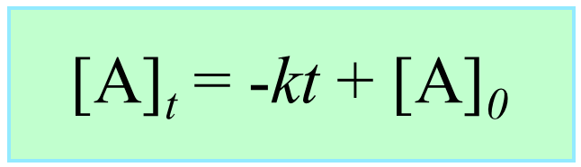
[A] = –kt + [A]₀

 

Integrating the Rate Law of First-Order Reaction

The rate law for a first-order reaction can be written as:

 

A → Products

Rate = k[A]¹

 

The rate is the change of concentration over time and therefore, the rate law cab be written as:

 

\[ – \frac{{\Delta [{\rm{A}}]}}{{\Delta t}}\; = \,k[{\rm{A}}]\]

 

The differential form of this equation is:

                                                                                      

\[\begin{array}{l} – \frac{{d[{\rm{A}}]}}{{dt}}\; = \,k[{\rm{A}}]\\ – \frac{{d[{\rm{A}}]}}{{[{\rm{A}}]}}\; = \,kdt\end{array}\]

 

And integrating the differential rate law, we obtain the integrated rate law for the zero-order reactions:

                                                                                 

\[\int_{{{[{\rm{A}}]}_0}}^{[{\rm{A}}]} {\frac{{d[{\rm{A}}]}}{{[{\rm{A}}]}}} \; = \, – \int_0^t {kdt} \]

                                               

\[\left[ {\ln [{\rm{A}}]} \right]_{{{[{\rm{A}}]}_0}}^{[{\rm{A}}]}\; = \, – k[t]_0^t\]

ln [A] – ln [A]₀ = –kt

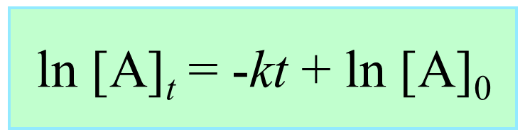
ln [A] = –kt + ln [A]₀

 

Integrating the Rate Law of First-Order Reaction

This time we write the rate law for a second-order reaction where the concentration of A is squared:

 

A → Products

Rate = k[A]²

 

The rate is the change of concentration over time and therefore, the rate law cab be written as:

 

\[ – \frac{{\Delta [{\rm{A}}]}}{{\Delta t}}\; = \,k{[{\rm{A}}]^2}\]

 

The differential form of this equation is:

                                                                                      

\[\begin{array}{l} – \frac{{d[{\rm{A}}]}}{{dt}}\; = \,k{[{\rm{A}}]^2}\\ – \frac{{d[{\rm{A}}]}}{{{{[{\rm{A}}]}^2}}}\; = \,kdt\end{array}\]

 

And integrating the differential rate law, we obtain the integrated rate law for the zero-order reactions:

                                                                                  

\[\int_{{{[{\rm{A}}]}_0}}^{[{\rm{A}}]} {\frac{{d[{\rm{A}}]}}{{{{[{\rm{A}}]}^2}}}} \; = \, – k\int_0^t {dt} \]

 

Solving this integral gives:

 

\[\int_{{{[{\rm{A}}]}_0}}^{[{\rm{A}}]} {\frac{{d[{\rm{A}}]}}{{{{[{\rm{A}}]}^2}}}} \; = \,\left( { – \frac{1}{{{{[{\rm{A}}]}_t}}}\; + \,{\rm{constant}}} \right)\; – \,\left( { – \frac{1}{{{{[{\rm{A}}]}_0}}}\; + \,{\rm{constant}}} \right)\; = \,\frac{1}{{{{\left[ {\rm{A}} \right]}_0}}}\, – \,\frac{1}{{\left[ {\rm{A}} \right]}}\;\,\]

 

Therefore,

                                                                                      

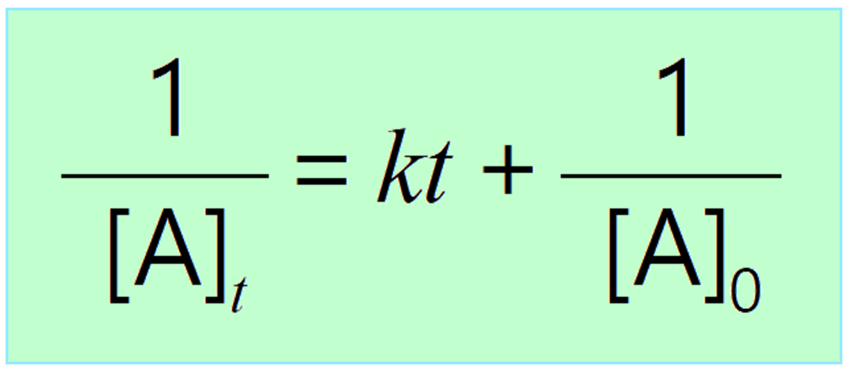
\[\frac{1}{{\left[ {\rm{A}} \right]}}\; – \,\frac{1}{{{{\left[ {\rm{A}} \right]}_0}}}\, = \;kt\]

 

And rearranging this equation, we get the integrated rate laws for second-order reactions in a familiar form:

 

 

This is how the integrated rate laws are obtained. You are likely not going to know how to do this in a typical general chemistry class where the emphasis will be on using the equations and graphs of the rate laws. Nonetheless, it is still an interesting question to discuss in the kinetics chapter.

                        

Here is a 77-question, Multiple-Choice Quiz on Chemical Kinetics:

                              

Check Also

• Reaction Rate
• Rate Law and Reaction Order
• How to Determine the Reaction Order
• Integrated Rate Law
• The Half-Life of a Reaction
• Determining the Reaction Order Using Graphs
• Units of Rate Constant k
• Activation Energy
• The Arrhenius Equation
• Chemical Kinetics Practice Problems